
티스토리 뷰
[논문 리뷰] BiSeNet V2: Bilateral Network with Guided Aggregation for Real-time Semantic Segmentation
감자보이 2021. 8. 22. 22:47Semantic segmentation분야에서
높은 accuracy와 적은 inference time을 동시에 잡은 Network
Abstract
semantic segmentation 분야의 경우 low-level detail과 high-level semantics가 중요하다.
기존의 논문들은 inference 속도를 향상시키기 위해 low-level detail을 포기하게 된다. 본 논문에서는 spatial detail과 categorical semantics를 모두 충족시키는 네트워크를 제안하며 real-time으로 semantic segmentation을 진행한다.
Detail branch에서는 넓은 channel과 얕은 layer를 이용해 high resolution을 얻고,
Semantic branch에서는 좁은 channel과 깊은 layer를 쌓아 high level의 semantic context를 얻을 수 있다.
이 두가지 branch를 적절하게 fuse할 수 있도록 Guided Aggregation Layer를 디자인했다.
NVIDIA GeForce GTX1080 Ti에서 input 크기 2048 X 1024를 이용해 156 FPS의 속도로 inference를 달성했으며 Cityscape test에서 Mean IOU를 72.6%를 달성했다.
Introduction
semantic segmentation은 각 픽셀마다 의미있는 class로 분류하는 작업이다. 이 기술은 컴퓨터 비전에서
핵심적인 부분 중 하나이며, scene understanding, autonomous driving, human-machine interaction 등에서 적용할 수 있다. 딥러닝이 발전됨에 다라 semantic segmentation의 정확도가 향상되었다. 하지만 inference 속도를 위해 low level detail을 포기하거나, high accuracy를 위해 inference 속도를 포기하는 방식만 존재했다.
따라서 이 논문에서는 두 가지를 모두 다루는 Bilateral Segmentation Network를 제안한다.
Semantic Branch
- categorical semantics
Detail Branch
- spatial detail
Guided Aggregation Layer
- Semantic Branch와 Detail Branch를 효과적으로 결합
booster
- inference complexity를 증가시키지 않고 성능을 향상하기 위해 추가
이전 버전에 비해 훨씬 간단하게 구성했으며 time-consuming이 존재하는 cross-layer connection을 제거했다. 또한 전체적인 아키텍처를 더욱 compact하게 새로 디자인했으며 이에 따라 성능도 더욱 향상되었다.
Core Concepts of BiSeNet V2
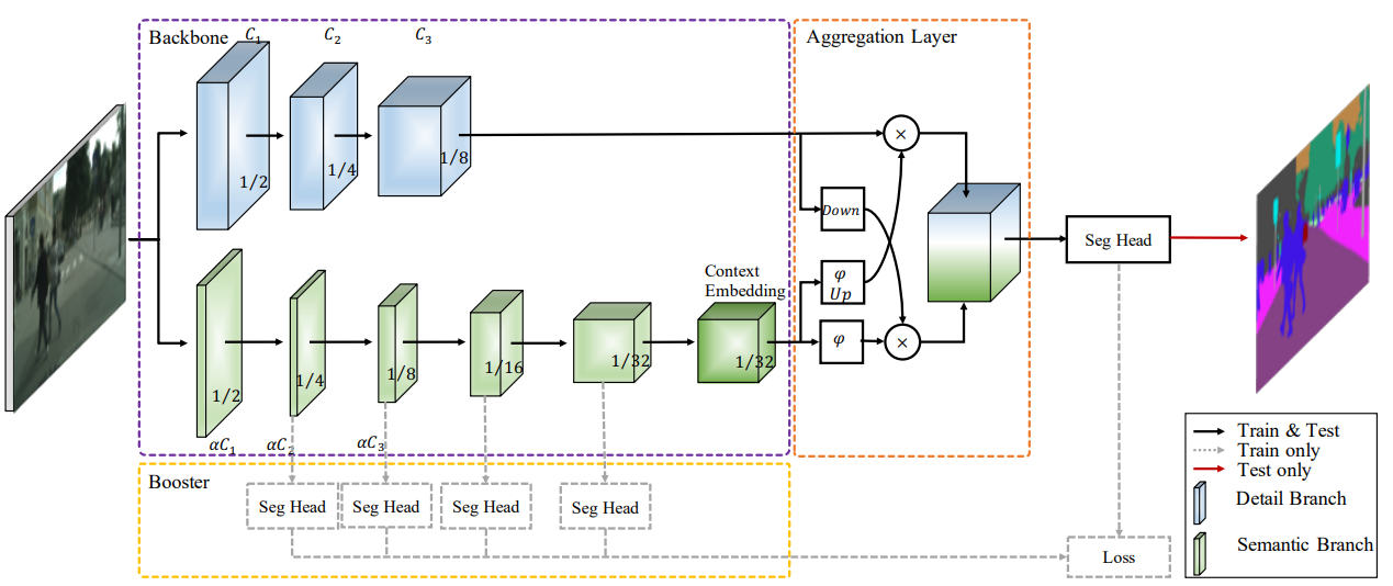
- Detail Branch
- low-level의 정보들이 담겨야 하므로 풍부한 channel 양을 가져야 한다. 따라서 채널 양은 많게 하면서 Layer의 수를 줄인다. 넓은 spatial size를 가지고 있으므로 residual connection을 진행하지 않는다.
- Semantic Branch
- Detail branch와는 반대로 적은 채널 양을 가지며 layer를 깊게 쌓는다. 이때 넓은 receptive field 넓히고 feature representation의 level을 높이기 위해 fast-down sampling 방법을 이용한다.
- Aggregation Layer
- 위 두 가지 branch를 merge 하기 위한 layer이다. semantic branch에서 fast-down sampling을 사용했기 때문에 detail branch에 비해 output이 작다. 따라서 semantic branch의 output feature map을 upsampling 한다. 이후 각각 element-wise product를 진행한 후 더한다.
receptive field가 클수록 공간적 정보가 풍부해지며 계산 시간이 줄어들어 Real time-segmentation에서는 필수적이다.
Bilateral Segmentation Network
Bisenet의 구체적인 구조를 설명한다.
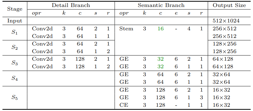
- Detail Branch
- 총 3개의 layer로 이루어져 있으며 각각 convolution과 batch normalization, 그리고 ReLu 활성화 함수가 포함되어있다.
- 최종적으로 input의 1/8 크기의 feature map을 뽑을 수 있다.
- Semantic Branch
- Semantic Branch는 Stem Block과 Context Embedding Block, Gather and Expansion Layer 구조를 이용한다.- Stem Block
- 서로 다른 방식의 downsampling을 진행한 이후에 두 branch를 concat 한다. 다음과 같은 전략을 사용함으로써 computation cost를 줄이고 효과적으로 feature를 뽑을 수 있었다.
- Context Embedding Block
- global contextual 정보를 효율적으로 얻기 위해서 average pooling과 resisual connection을 사용했다.
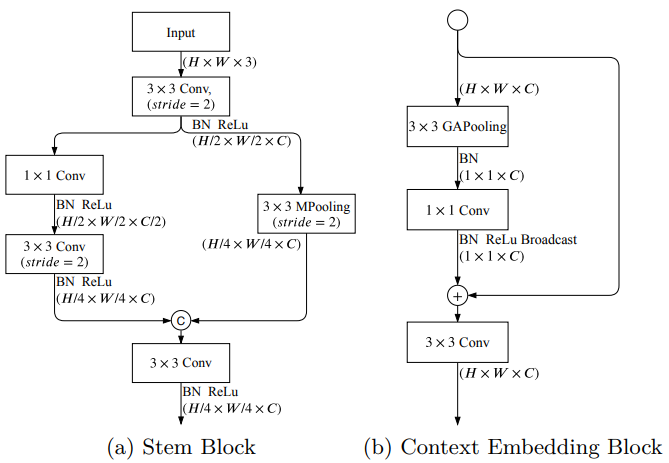
Stem Block과 Context Embedding Block의 구조 - Gather and Expansion Layer
- depth-wise convolution을 이용하며 마지막에 1X1 convolution을 이용해 depth-wise conv의 output을 projection 시킨다.
- 기존 mobilenet v2의 구조와는 다르게 GE layer는 3X3 convolution을 하나 더 사용함으로써 더 좋은 feature quality를 얻을 수 있었다.
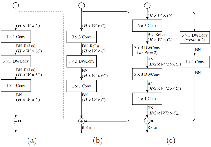
a는 mobilenet v2에서 제안된 구조이며 b,c는 본 논문에서 제안된 GE구조. - Booster Training Strategy
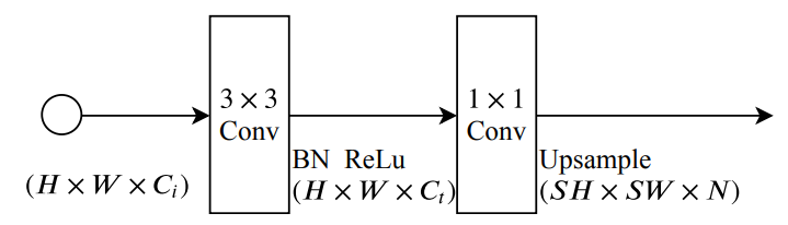
- segmentation accuracy를 위해서 booster strategy를 도입했다. 트레이닝 시, feature representation을 향상시키며 inference 시에는 computation cost는 그리 크지 않다. semantic branch 사이사이에 삽입시킨다.
Booster 구조
- segmentation accuracy를 위해서 booster strategy를 도입했다. 트레이닝 시, feature representation을 향상시키며 inference 시에는 computation cost는 그리 크지 않다. semantic branch 사이사이에 삽입시킨다.
- Stem Block
depth-wise convolution은 각 채널마다 독립적인 filter(커널)을 가지고 있다. 따라서 입력과 출력의 채널 수가 동일하고 각 채널마다 고유의 spatial 정보를 학습할 수 있는 장점을 가지고 있다.
Experimental Result
Cityscapes dataset을 사용했으며 training시에는 2975개, validation 시 500개, test시에는 1525개의 data를 사용했다. dataset의 resolution은 2048 X 1024이다.
Loss의 경우 논문에서는 따로 언급이 되어있지 않지만 공식 github를 통해서 Cross Entopy loss를 사용하는 것으로 확인됐다.
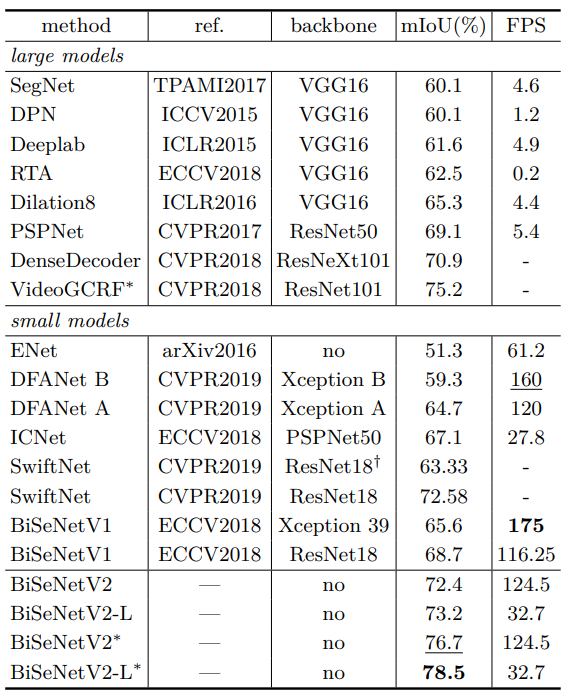
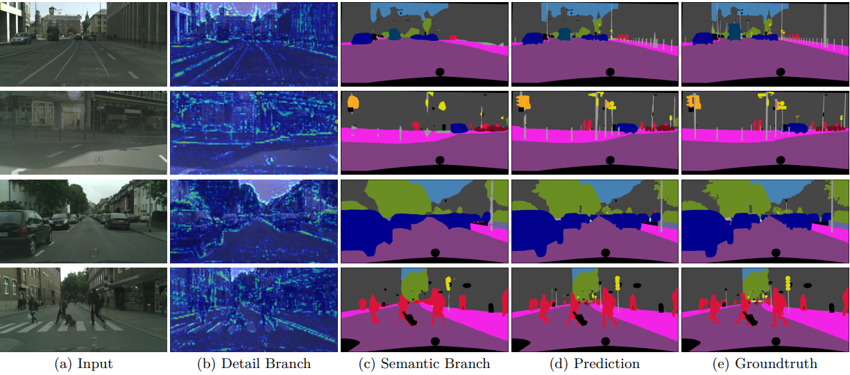
기존 SOTA 논문들에 비해 높은 mIoU와 FPS를 얻은 것을 확인할 수 있었다.
현재 이 segmentation output을 이용해서 연구를 진행하고 있다. 곧 새로운 연구 결과로 포스트를 올려볼 예정이다.
reference
'연구 일지 > 논문 리뷰' 카테고리의 다른 글
- Total
- Today
- Yesterday
- 연구
- 딥러닝
- 논문
- 자율주행
- opencv
- prediction
- 컴퓨터비전
- slam
- Camera
- 논문구현
- Visual Odometry
- 리뷰
- mobile robot
- path planning
- segmentation
- Vision
- 논문리뷰
- 블로그 #작성요령 #시작
- estimation
- bts
- 아르떼뮤지엄 #여수 #여행
- depth
| 일 | 월 | 화 | 수 | 목 | 금 | 토 |
|---|---|---|---|---|---|---|
| 1 | 2 | 3 | ||||
| 4 | 5 | 6 | 7 | 8 | 9 | 10 |
| 11 | 12 | 13 | 14 | 15 | 16 | 17 |
| 18 | 19 | 20 | 21 | 22 | 23 | 24 |
| 25 | 26 | 27 | 28 | 29 | 30 | 31 |